Linear and Nonlinear Regression

Image source: https://www.freepik.com

Introduction

In this blog, we’re going to solve the House Prices Prediction problem with linear and nonlinear regression models. Regression is one of the most important machine learning (ML) algorithm, it is very straightforward and intuitive. It is usually the first algorithm we encounter in our machine learning journey, so let’s conquer it together!

We’re going to cover the following regression models in this post:

• Linear Models
  • Linear Regression
  • Ridge Regression
  • Lasso Regression
  • Elastic Net Regression
• Nonlinear Models
  • Polynomial Regression
  • Artificial Neural Network

Data

The dataset used in this blog is downloaded from Kaggle USA Housing. The whole dataset is about 5000 rows and 7 columns stored in the csv format, a local downloaded copy could be found as USA_Housing.csv file.

Exploratory Data Analysis

We first conduct some exploratory data analysis. We’re going to use the pandas library to load and process data, and use the matplotlib and seaborn library for data visualizations.

Import Libraries

import numpy as np
import pandas as pd
import matplotlib.pyplot as plt
import hvplot.pandas
import seaborn as sns
from sklearn.model_selection import train_test_split

Load Data

housing_df = pd.read_csv('data/USA_Housing.csv')
housing_df.head()

Table 1: Samples of the dataset

	Avg. Area Income	Avg. Area House Age	Avg. Area Number of Rooms	Avg. Area Number of Bedrooms	Area Population	Price	Address
0	79545.458574	5.682861	7.009188	4.09	23086.800503	1.059034e+06	208 Michael Ferry Apt. 674\nLaurabury, NE 3701...
1	79248.642455	6.002900	6.730821	3.09	40173.072174	1.505891e+06	188 Johnson Views Suite 079\nLake Kathleen, CA...
2	61287.067179	5.865890	8.512727	5.13	36882.159400	1.058988e+06	9127 Elizabeth Stravenue\nDanieltown, WI 06482...
3	63345.240046	7.188236	5.586729	3.26	34310.242831	1.260617e+06	USS Barnett\nFPO AP 44820
4	59982.197226	5.040555	7.839388	4.23	26354.109472	6.309435e+05	USNS Raymond\nFPO AE 09386

As we can see in the Table 1, there are 6 numeric columns represents the average area income, house age, number of rooms, number of bedrooms, area population and price, respectively. There is only 1 textual column, keeps the house address.

Our goal is modeling the house price, so it should be the dependent variable in the regressions, and all the other columns should be treated as the independent variable.

We now have a quick examination of the descriptive statistics.

housing_df.describe()

	Avg. Area Income	Avg. Area House Age	Avg. Area Number of Rooms	Avg. Area Number of Bedrooms	Area Population	Price
count	5000.000000	5000.000000	5000.000000	5000.000000	5000.000000	5.000000e+03
mean	68583.108984	5.977222	6.987792	3.981330	36163.516039	1.232073e+06
std	10657.991214	0.991456	1.005833	1.234137	9925.650114	3.531176e+05
min	17796.631190	2.644304	3.236194	2.000000	172.610686	1.593866e+04
25%	61480.562388	5.322283	6.299250	3.140000	29403.928702	9.975771e+05
50%	68804.286404	5.970429	7.002902	4.050000	36199.406689	1.232669e+06
75%	75783.338666	6.650808	7.665871	4.490000	42861.290769	1.471210e+06
max	107701.748378	9.519088	10.759588	6.500000	69621.713378	2.469066e+06

In order to have better insights on the variables, we further visualize the data distributions as follows.

sns.pairplot(housing_df)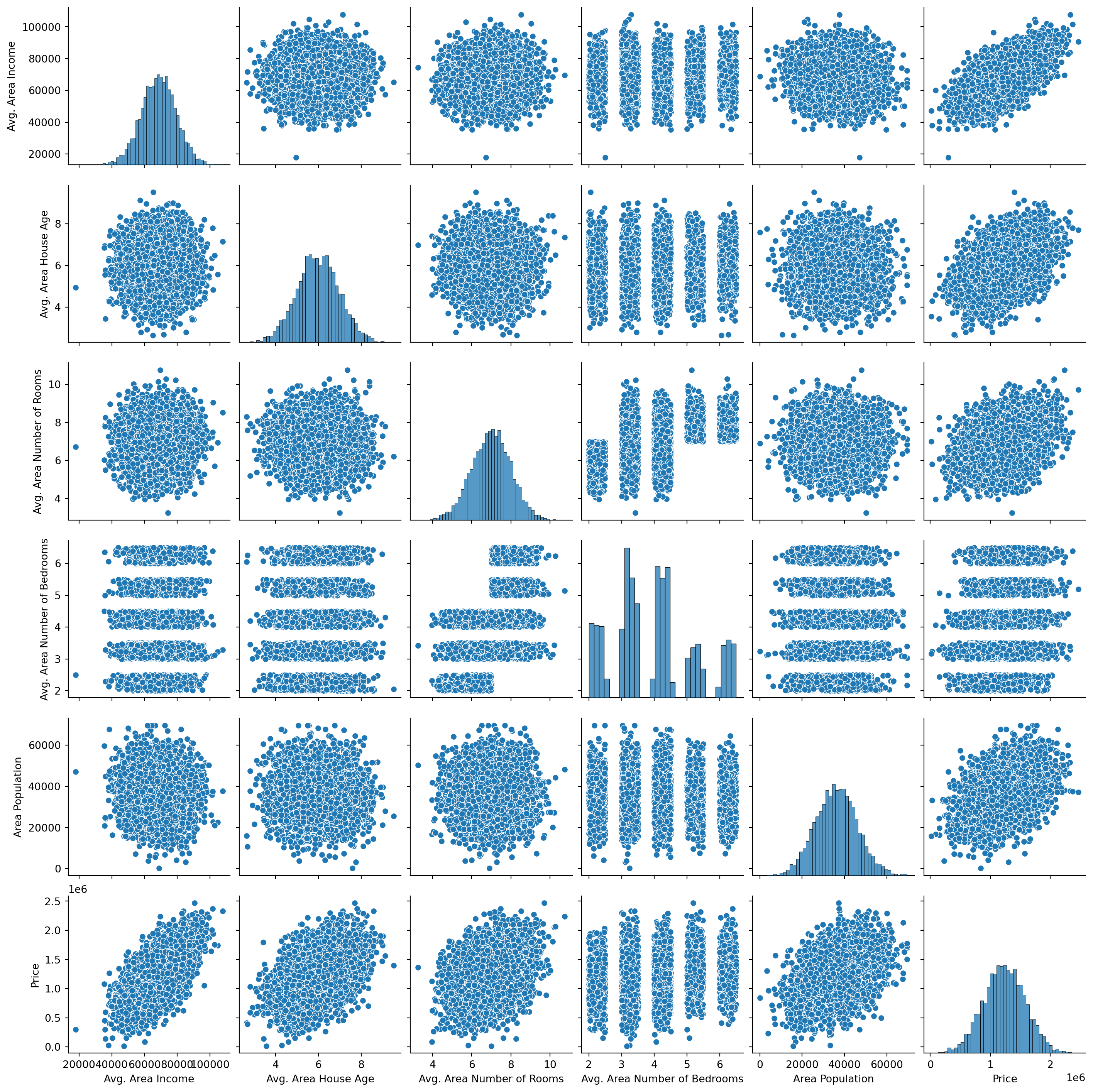

Figure 1: The data distribution of variables

As Table 1 shows, most of our variables are normal distributed, except for the average number of bedrooms, there is clearly some linear trends between the dependent variable Price and other variables.

housing_df.hvplot.hist('Price')
plt.show()

We further examine the relations between the dependent variable, for instance, we plot the relationship between Price and Avg. Area Income interactively as below.

housing_df.hvplot.scatter(x='Avg. Area Income', y='Price')
plt.show()

Correlation Coefficient

axes_arr = sns.heatmap(
  housing_df[[
    col for col in housing_df.columns if col not in ["Address","Price"]
    ]].corr()
  )
plt.show()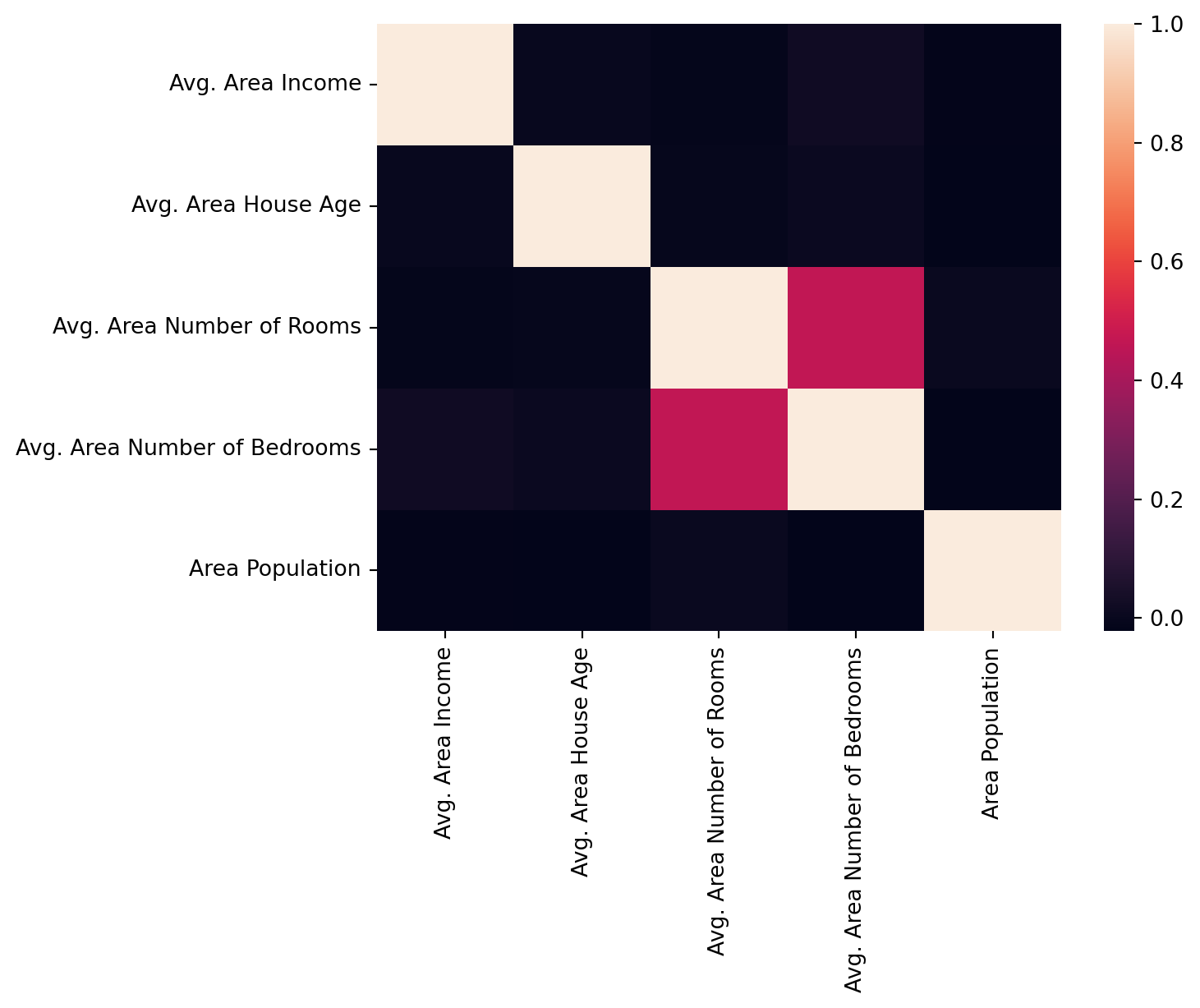

Figure 2: The plot of Correlation Coefficient

As it is clearly shown in Figure 2, the Avg. Area Income is most correlated with Price, followed by Avg. Area House Age, Area Population, Avg. Area Number of Rooms. The variable Avg. Area Number of Bedrooms has the smallest correlation score at 0.17. Thus, we will include all these variables in the modeling section.

Preprocessing

In order to fully exploit the linear regression, especially for better interpretability, we have to check if our data satisfies some criteria for linear regression application. For example:

• Linear Assumption. The linear regression models assume there are linear relationship between the dependent variable and independent variables.

• Noise Removal. The noises (i.e., missing value, outliers) in data could potentially impair the model performance, we have to remove these noise before modeling.

• Gaussian Distribution. Linear regression works well with data comply with gaussian distribution. For those not, we have to apply data transformation techniques (e.g., log transform, BoxCox) to make the data more gaussian distributed.

• Variable Scaling. If variable values are at different magnitudes, we need to scale them to the same magnitudes by using standardization or normalization.

We have already tested the linear assumption and gaussian distribution in the exploratory data analysis section. And the data is relatively clean, noise is not a problem, however, the value of variables are at different magnitude, we will perform re-scaling before modeling steps.

from sklearn.preprocessing import StandardScaler
from sklearn.pipeline import Pipeline
pipeline = Pipeline([
    ('std_scalar', StandardScaler())
])

X = housing_df[[
    col for col in housing_df.columns if col not in ["Address","Price"] 
    ]]
y = housing_df['Price'].to_numpy()

X_scaled = pipeline.fit_transform(X)

pd.DataFrame(X_scaled).describe()

	0	1	2	3	4
count	5.000000e+03	5.000000e+03	5.000000e+03	5.000000e+03	5.000000e+03
mean	-2.167155e-17	4.263256e-18	-4.135359e-16	-2.088996e-16	-3.041123e-16
std	1.000100e+00	1.000100e+00	1.000100e+00	1.000100e+00	1.000100e+00
min	-4.765584e+00	-3.361975e+00	-3.730214e+00	-1.605598e+00	-3.626413e+00
25%	-6.664724e-01	-6.606490e-01	-6.846171e-01	-6.817833e-01	-6.810902e-01
50%	2.075434e-02	-6.852312e-03	1.502401e-02	5.564767e-02	3.616311e-03
75%	6.756386e-01	6.794590e-01	6.742146e-01	4.122077e-01	6.748621e-01
max	3.670725e+00	3.572745e+00	3.750297e+00	2.041039e+00	3.371219e+00

Data Split

Before the modeling steps, we first the dataset into train, validation and test split. We will use sklearn to perform this task.

X_train, X_test, y_train, y_test = train_test_split(X_scaled, y, test_size=0.2, random_state=666)

print(f"The size of train split: {len(X_train)}")
print(f"The size of test split: {len(X_test)}")

The size of train split: 4000
The size of test split: 1000

Modeling

In this section, we will first introduce the model evaluation metrics and then modeling the data using various of regression algorithms.

Evaluation

There are several popular evaluation metrics which are widely used in regression problem.

RMSE

Root Mean Squared Error (RMSE) is the square root of the mean of the squared errors:

\operatorname{RMSE}= \sqrt{\frac{1}{n}\sum_{i=1}^n(\hat{y_i} - y_i)^2}

where,

• x_i = independent variable of each data point

• y_i = dependent variable of each data point

• \bar{y} = mean of y value

• \hat{y_i} = the predict y value base on x

R-Squared (R²) Score

R^2 describes the proportion of dependent variance explained by the regression model¹. It could be denoted by the following equation.

\operatorname{R^2} = \frac{SSR}{SST}

where,

• SSR = \sum_{i=1}^n \left(\hat{y_i} - \bar{y}\right)^2

• \operatorname{SST} = \sum_{i=1}^n \left(y_i - \bar{y}\right)^2

Evaluation using Sklearn

from sklearn import metrics

def print_evaluate(true, predicted):  
    rmse = np.sqrt(metrics.mean_squared_error(true, predicted))
    r2_square = metrics.r2_score(true, predicted)
    print('RMSE:', rmse)
    print('R2 Square', r2_square)
    print('__________________________________')
    
def evaluate(true, predicted):
    rmse = np.sqrt(metrics.mean_squared_error(true, predicted))
    r2_square = metrics.r2_score(true, predicted)
    return rmse, r2_square

Linear Models

Linear Regression

We now train a linear regression model using sklearn library.

Training

from sklearn.linear_model import LinearRegression
linear_md = LinearRegression()
linear_md.fit(X_train, y_train)

LinearRegression()

In a Jupyter environment, please rerun this cell to show the HTML representation or trust the notebook.
On GitHub, the HTML representation is unable to render, please try loading this page with nbviewer.org.

After the fit, we completed the model train. The next step is verify the fitting result and evaluate the model performance.

Interpreting

We can access the model intercept and coefficients using the sklearn API:

print(f"The intercept is: {linear_md.intercept_}")
coef_df = pd.DataFrame(linear_md.coef_, X.columns, columns=['Coefficient'])
coef_df

The intercept is: 1232604.4076491522

	Coefficient
Avg. Area Income	230982.846988
Avg. Area House Age	162799.384625
Avg. Area Number of Rooms	122310.560876
Avg. Area Number of Bedrooms	2376.796391
Area Population	151198.049691

Prediction

Predict using the model

pred = linear_md.predict(X_test)
pd.DataFrame({'True Values': y_test, 'Predicted Values': pred}).hvplot.scatter(x='True Values', y='Predicted Values')

The residual histogram is plotted as following:

pd.DataFrame({'Error Values': (y_test - pred)}).hvplot.kde()

Performance

pred_train = linear_md.predict(X_train)
pred_test = linear_md.predict(X_test)
print(f"The train set performance:\n")
print_evaluate(y_train, pred_train)
print(f"The test set performance:\n")
print_evaluate(y_test, pred_test)

The train set performance:

RMSE: 100782.52384490197
R2 Square 0.9178558419818683
__________________________________
The test set performance:

RMSE: 102440.81503100201
R2 Square 0.9184591335733732
__________________________________

Ridge Regression

Ridge regression is a type of regularized linear regression, it imposes a penalty on the size of the coefficients, it could be expressed using the equation²:

\min_{w} || X w - y||_2^2 + \alpha ||w||_2^2

The parameter \alpha controls the amount of the penalty, the larger the \alpha, the more penalty is imposed, the coefficient is more shrink to 0.

Similar to linear regression, we do modeling and evaluation using the ridge regression as following:

from sklearn.linear_model import Ridge
ridge_md = Ridge(alpha = 20,  solver='cholesky',  tol=0.0001, random_state=666)
ridge_md.fit(X_train, y_train)

Ridge(alpha=20, random_state=666, solver='cholesky')

In a Jupyter environment, please rerun this cell to show the HTML representation or trust the notebook.
On GitHub, the HTML representation is unable to render, please try loading this page with nbviewer.org.

pred_train = ridge_md.predict(X_train)
pred_test = ridge_md.predict(X_test)
print(f"The train set performance:\n")
print_evaluate(y_train, pred_train)
print(f"The test set performance:\n")
print_evaluate(y_test, pred_test)

The train set performance:

RMSE: 100798.00734362529
R2 Square 0.9178305999732655
__________________________________
The test set performance:

RMSE: 102413.21431785727
R2 Square 0.9185030668996456
__________________________________

Lasso Regression

Ridge regression is another type of regularized linear regression, specifically, using L1 regularization. It adds the absolute value of the coefficient to the loss function as the penalty. Mathematically, it could be expressed using the equation³:

\min_{w} { \frac{1}{2n_{\text{samples}}} ||X w - y||_2 ^ 2 + \alpha ||w||_1}

The parameter \alpha is a constant which controls the amount of the penalty, the ||w||_1 is the \ell_1-norm of the coefficients.

Lasso Regression modeling and performance evaluation is performed bellow:

from sklearn.linear_model import Lasso

lasso_md = Lasso(alpha = 0.08, selection='random', positive=True, random_state=888)
lasso_md.fit(X_train, y_train)

Lasso(alpha=0.08, positive=True, random_state=888, selection='random')

In a Jupyter environment, please rerun this cell to show the HTML representation or trust the notebook.
On GitHub, the HTML representation is unable to render, please try loading this page with nbviewer.org.

pred_train = lasso_md.predict(X_train)
pred_test = lasso_md.predict(X_test)
print(f"The train set performance:\n")
print_evaluate(y_train, pred_train)
print(f"The test set performance:\n")
print_evaluate(y_test, pred_test)

The train set performance:

RMSE: 100782.52384504011
R2 Square 0.917855841981643
__________________________________
The test set performance:

RMSE: 102440.81373676285
R2 Square 0.9184591356337508
__________________________________

Elastic Net Regression

Elastic net regression is essentially a combination of Ridge and Lasso regression. As it adds two regularization term: L2 and L1 regularization which is used in Ridge and Lasso regression respectively. The trade-off between Ridge and Lasso allows elastic net regression picks up the advantages of these two models. The lost function is written as⁴:

\min_{w}{\frac{1}{2n_{samples}} \big|\big|X w - y\big|\big|_2 ^ 2 + \alpha \rho \big|\big|w\big|\big|_1 + \frac{\alpha(1-\rho)}{2} \big|\big|w\big|\big|_2 ^ 2}

The parameters alpha \alpha and l1_ratio \rho could be decided by cross-validation.

from sklearn.linear_model import ElasticNet

enet_md = ElasticNet(alpha=0.08, l1_ratio=0.9, selection='random', random_state=666)
enet_md.fit(X_train, y_train)

ElasticNet(alpha=0.08, l1_ratio=0.9, random_state=666, selection='random')

In a Jupyter environment, please rerun this cell to show the HTML representation or trust the notebook.
On GitHub, the HTML representation is unable to render, please try loading this page with nbviewer.org.

pred_train = enet_md.predict(X_train)
pred_test = enet_md.predict(X_test)
print(f"The train set performance:\n")
print_evaluate(y_train, pred_train)
print(f"The test set performance:\n")
print_evaluate(y_test, pred_test)

The train set performance:

RMSE: 100821.89673708729
R2 Square 0.9177916466289507
__________________________________
The test set performance:

RMSE: 102411.86137925804
R2 Square 0.9185052201299478
__________________________________

Nonlinear Models

All the model introduce above are belong to linear category. However, linear models is not designed to capture nonlinear trends in the data. If the relationship between dependent variable and independent variables are not linear, we have to apply nonlinear models. Among various options, polynomial regression and artificial neural network are the popular ones.

Polynomial Regression

Polynomial regression is a extension to linear regression by introducing polynomial terms. Recall the linear regression model looks like⁵:

\hat{y}(w, x) = w_0 + w_1 x_1 + w_2 x_2

However, we can add quadratic term to the previous equation to fit a parabola instead of a plane, then it looks like:

\hat{y}(w, x) = w_0 + w_1 x_1 + w_2 x_2 + w_3 x_1 x_2 + w_4 x_1^2 + w_5 x_2^2

We can new image creating a set of features as:

z = [x_1, x_2, x_1 x_2, x_1^2, x_2^2]

Then, we combine the features and coefficients linearly, and get the following:

\hat{y}(w, z) = w_0 + w_1 z_1 + w_2 z_2 + w_3 z_3 + w_4 z_4 + w_5 z_5

Modeling

from sklearn.preprocessing import PolynomialFeatures
poly_md = PolynomialFeatures(degree=2)

X_train_2_d = poly_md.fit_transform(X_train)
X_test_2_d = poly_md.transform(X_test)

linear_reg = LinearRegression()
linear_reg.fit(X_train_2_d, y_train)

LinearRegression()

In a Jupyter environment, please rerun this cell to show the HTML representation or trust the notebook.
On GitHub, the HTML representation is unable to render, please try loading this page with nbviewer.org.

Performance

pred_train = linear_reg.predict(X_train_2_d)
pred_test = linear_reg.predict(X_test_2_d)
print(f"The train set performance:\n")
print_evaluate(y_train, pred_train)
print(f"The test set performance:\n")
print_evaluate(y_test, pred_test)

The train set performance:

RMSE: 100640.24459847226
R2 Square 0.9180876115116245
__________________________________
The test set performance:

RMSE: 102720.10827633881
R2 Square 0.918013903645979
__________________________________

Artificial Neural Network

Artificial Neural Network is a very powerful model to fit linear and nonlinear data. In this section, we will use pytorch framework to build a artificial neural network to predict the house prices. Similar to previous models, we start from build the network, then train the models and report the performance in the end.

Network Construction

Import the libraries:

import torch
import torch.nn as nn
import torch.nn.functional as F
from torch.utils.data import Dataset, DataLoader

Define the HousePriceDataset by extending pytorch’s Dataset class, it is simply convert the numpy array to pytorch tensor.

class HousePriceDataset(Dataset):
  def __init__(self, X, Y):
    self.X = torch.tensor(X, dtype=torch.float32)
    self.y = torch.tensor(Y, dtype=torch.float32)

  def __len__(self):
    return len(self.X)

  def __getitem__(self, index):
    return (self.X[index], self.y[index])

We new create the DataLoader objects, which load the data in batch to feed into the neural network.

train_ds = HousePriceDataset(X_train, y_train)
test_ds = HousePriceDataset(X_test, y_test)
trainloader = DataLoader(train_ds, batch_size=32, shuffle=True,
                         num_workers=2, drop_last=True)
testloader = DataLoader(test_ds, batch_size=32, shuffle=True, num_workers=2,
                        drop_last=True)

The code below creates the neural network. It consist of several feed-forward layer with dropout regularization and use RELU as activate function. Each layer is like a linear regression, and the activate function map the output into the nonlinear space. That is why neural network could be used as a nonlinear regressor.

class MLP(nn.Module):
  def __init__(self):
    super(MLP, self).__init__()
    self.layers = nn.Sequential(
        nn.Linear(5, 64),
        nn.Dropout(0.2),
        nn.ReLU(),
        nn.Linear(64, 128),
        nn.Dropout(0.2),
        nn.ReLU(),
        nn.Linear(128, 64),
        nn.Dropout(0.2),
        nn.ReLU(),
        nn.Linear(64, 1)
    )
  def forward(self, x):
    return self.layers(x)

Training

We first implement the evaluate function which loads the test data, pass it to the pre-trained model and reports the MSE and R^2 as performance metrics.

def evaluate(model):
    pred_list = []
    label_list = []
    loss_list = []
    loss_function = nn.MSELoss()
    model.eval()
    for i, data in enumerate(testloader):
        # Get inputs
        inputs, targets = data
        # Perform forward pass
        outputs = model(inputs)
        outputs = outputs.squeeze(-1)
        loss = loss_function(outputs, targets)
        loss_list.append(loss.item())
        pred_list.append(outputs.detach().numpy())
        label_list.append(targets.numpy())

    avg_loss = sum(loss_list) / len(testloader)
    pred_np = np.vstack(pred_list)
    label_np = np.vstack(label_list)
    avg_r2 = metrics.r2_score(pred_np, label_np)
    return (avg_loss, avg_r2)

The then implements the train function to manage the whole training process, it initialize the neural network, data loader, loss function and the optimizer. Data is passed forward in the network and errors are propagated backward in the network.

def train():
    mlp = MLP()
    torch.manual_seed(666)
    trainloader = DataLoader(train_ds, batch_size=32, shuffle=True,
                             num_workers=2)
    loss_function = nn.MSELoss()
    optimizer = torch.optim.Adam(mlp.parameters(), lr=6e-4)
    n_epochs = 150
    mlp.train()
    train_loss_list = []
    train_r2_list = []
    test_loss_list = []
    test_r2_list = []
    for epoch in range(n_epochs):
        pred_list = []
        label_list = []
        loss_list = []
        for i, data in enumerate(trainloader):
            inputs, targets = data
            # Zero the gradients
            optimizer.zero_grad()
            # Perform forward pass
            outputs = mlp(inputs)
            outputs = outputs.squeeze(-1)
            # Compute loss
            loss = loss_function(outputs, targets)
            # Perform backward pass
            loss.backward()
            # Perform optimizationd
            optimizer.step()
            # Print statistics    
            pred_list.append(outputs.detach().numpy())
            label_list.append(targets.numpy())
            loss_list.append(loss.item())

        avg_loss = sum(loss_list) / len(trainloader)
        pred_np = np.vstack(pred_list)
        label_np = np.vstack(label_list)
        avg_r2 = metrics.r2_score(pred_np, label_np)
        train_loss_list.append(avg_loss)
        train_r2_list.append(avg_r2)
        test_loss, test_r2 = evaluate(mlp)
        test_loss_list.append(test_loss)
        test_r2_list.append(test_r2)
        print(f"epoch: {epoch}, test_loss: {test_loss}, test_r2: {test_r2}")
    print('Training process has finished.')
    return mlp, train_loss_list, train_r2_list, test_loss_list, test_r2_list

Start the training process:

model, train_loss_list, train_r2_list, test_loss_list, test_r2_list = train()

Evaluation

Similar to previous model, we reports the RMSE and R^2 of the test set as the evaluation metrics:

test_loss, test_r2 = evaluate(model)
print(f"The test set performance:\n")
rmse = np.sqrt(test_loss)
print('RMSE:', rmse)
print('R2 Square', test_r2)
print('__________________________________')

The test set performance:

RMSE: 102623.80293089902
R2 Square 0.9047423651342836
__________________________________

train_loss = train_loss_list
val_loss = test_loss_list
train_r2 = train_r2_list
val_r2 = test_r2_list

Further, we can visualize the the RMSE of the train and test split during the whole training process, which is shown as follows:

# Draw loss plot
import matplotlib.pyplot as plt
plt.figure(figsize = (6,6))
plt.plot(train_loss, label='Training Loss')
plt.plot(val_loss, label='Validation Loss')
plt.xlabel('Batch')
plt.ylabel('Loss')
plt.legend()
plt.title('Loss')
plt.show()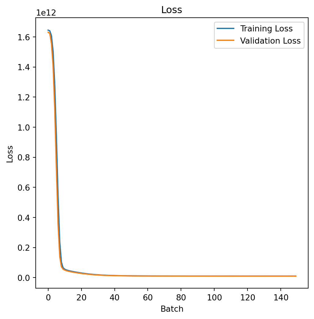

The R^2 of the train and test split during the whole training process is shown as follows:

# Draw accuracy plot
plt.figure(figsize = (6,6))
plt.plot(train_r2[10:], label='Training Accuracy')
plt.plot(val_r2[10:], label='Validation Accuracy')
plt.xlabel('Batch')
plt.ylabel('Accuracy')
plt.legend()
plt.title('Accuracy')
plt.show()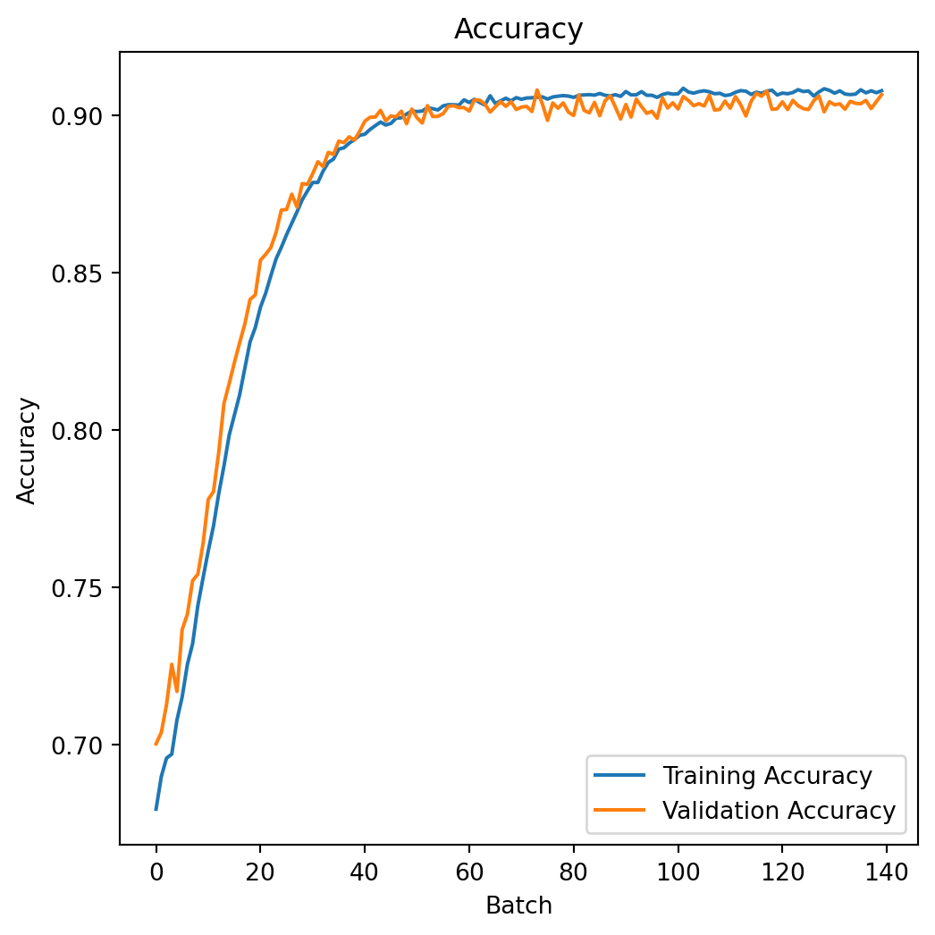

Discussion and Conclusion

In this blog, we applied 4 linear regression models and 2 nonlinear regression models in predicting the house price. Although trained on the same training set, these models vary in performance and have different characteristics in training.

Linear or nonlinear regression should I use? The choice between linear regression and nonlinear regression depends on the underlying relationship between the independent and dependent variables in your dataset. Here are some guidelines can be summarized from our previous experiments:

Linearity of the Relationship:

• Use linear regression when the relationship between the independent and dependent variables appears to be linear. Linear regression models assume a straight-line relationship, and they are suitable when the data points seem to follow a linear pattern.

• Use nonlinear regression when the relationship is not linear. If the data exhibits a curve, exponential growth, decay, or any other nonlinear pattern, a nonlinear regression model may be more appropriate.

Model Complexity:

• Linear regression models are simpler and easier to interpret. If a linear relationship adequately describes the data, it’s often preferable due to its simplicity.

• Nonlinear regression models can capture more complex relationships but may be harder to interpret. Be cautious about overfitting, where a model captures noise in the data rather than the underlying pattern.

As the house price data we used has a simple linear pattern, so, the performance is has no big difference than the nonlinear models. But it is much simple to implement and requires much less time and resource for training. In this kind of scenario, linear regression could be a good choice.

In summary, the decision to use linear or nonlinear regression depends on the characteristics of your data and the underlying relationship between variables.

Footnotes

1. https://en.wikipedia.org/wiki/Coefficient_of_determination

2. https://scikit-learn.org/stable/modules/linear_model.html#ridge-regression

3. https://scikit-learn.org/stable/modules/generated/sklearn.linear_model.Lasso.html#sklearn.linear_model.Lasso

4. https://scikit-learn.org/stable/modules/generated/sklearn.linear_model.ElasticNet.html#sklearn.linear_model.ElasticNet

5. https://scikit-learn.org/stable/modules/linear_model.html#polynomial-regression-extending-linear-models-with-basis-functions